Covariant derivatives and parallelism November 1, 2009
Posted by Akhil Mathew in differential geometry, MaBloWriMo.
Tags: connections, covariant derivatives, ordinary differential equations, parallelism
trackback
[Nobody should read this post without reading the excellent comments below. It turns out that thinking more generally (via connections on the pullback bundle) clarifies things. Many thanks to the (anonymous) reader who posted them. –AM, 5/16]
A couple of days back I covered the definition of a (Koszul) connection. Now I will describe how this gives a way to differentiate vector fields along a curve.
Covariant Derivatives
First of all, here is a minor remark I should have made before. Given a connection  and a vector field
  , the operation
  is linear in
  over smooth functions—thus it is a tensor (of type (1,1)), and the value at a point
  can be defined if is replaced by a tangent vector at . In other words, we get a map
  , where
  denotes the space of vector fields. We’re going to need this below.
Next, a curve  in the smooth manifold
  is an immersion
  , where
  is an interval in
  . We can talk about a vector field along to be a map
  such that
  lies above
  . An example is the derivative
  .
.
Now assume is given a connection . I claim that there is a unique operator  sending vector fields along to vector fields along such that:
- If is a vector field along and
 , then
  .Note that
 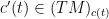 , by definition.
- If is the restriction of a vector field
 on , i.e.
  , then
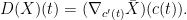
This operator is called the covariant derivative along . It is in fact a generalization of the usual directional derivative of vector fields in multivariable calculus, which occurs when you take the connection on  with all Christoffel symbols zero.
The first condition means we can, by multiplying by a cut-off function, assume is supported in some coordinate neighborhood  with coordinates
  . In particular, we may even assume that the image of is contained in by shrinking and using local uniqueness (which we prove below). Moreover, we can assume that is one-to-one by shrinking further.
Now, in the local case, we can write  , and
, and  , where
  . We can extend to
  . Let the Christoffel symbols of the connections be
  . We write write what
  looks like, and dive into the algebra. By linearity

This equals by the derivation-like identity for connections
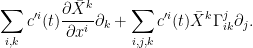
Shifting the indices, collecting terms, and using that is a restriction of gives that if we have such an operator , then
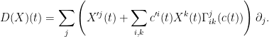
So we’re basically out of the woods—this expression depends only on . Thus we define  this way in local coordinates; it is easily checked that the conditions are satisfied locally, and one pieces together the local covariant derivatives to get the global ones. The fact that patching is legal follows from the uniqueness assertion and a partition of unity argument.
Parallelism
A vector field along the curve is said to be parallel if  . For instance, in the case of with the usual connection, this means that all the components are constant.
Now fix a curve starting at and ending at  , with interval
 ![{[0,1]}](https://s0.wp.com/latex.php?latex=%7B%5B0%2C1%5D%7D&bg=ffffff&fg=000000&s=0&c=20201002) .
.
Proposition 1 Given  , there is a unique parallel vector field along such that
  .
.
Indeed, we may assume that ![{c([0,1])}](https://s0.wp.com/latex.php?latex=%7Bc%28%5B0%2C1%5D%29%7D&bg=ffffff&fg=000000&s=0&c=20201002) is contained in a coordinate neigbhorhood, in which case it follows from the fundamental existence and uniqueness theorem on linear ODEs(!) and the local equation for a connection.
is contained in a coordinate neigbhorhood, in which case it follows from the fundamental existence and uniqueness theorem on linear ODEs(!) and the local equation for a connection.
Anyway, this means that we can define a map  as follows: for
  , choose a curve as above, and then take
  . It’s smooth because of the smoothness theorem on ODEs. It’s even linear because if
  correspond to
  , then
  corresponds to
  , etc.
The next result tells us what I have been insisting all along—that connections are about connecting different tangent spaces.
Proposition 2  is a linear isomorphism.
We just need to check that it’s one to one. This follows because the value of the vector field along at  determines its value along , because of the uniqueness theorem on ODEs again.
However, does depend on the curve . I believe the extent to which this dependence holds is measured by the holonomy groups, but I don’t (yet) understand what that’s all about, so I’ll let you read about it elsewhere.

[…] Covariant derivatives and parallelism […]
This proof is incorrect (as in some standard books too) because it overlooks the possibility that the map may not be locally immersive and the image could be extremely self-crossing: the very concept of “vector field along a parametric curve” is awkward to work with if stuck inside the manifold in cases when the parametric map is not locally immersive. So pull back to bundle with connection over the time interval and use the existence/uniqueness theorem on linear ODE to get the canonical framing by flat sections for the pullback. Sections of the pullback bundle are rigorous meaning of vector field along the parametric curve as well. Anyway, old-style differentiation relative to that framing of flat sections gives the construction, with all properties then easy to verify.
Thanks for pointing this out! However, I’m not sure I understand how this differs from defining a vector field along as a map
  (where
  is the parameter interval) – is this not the same as the pullback bundle? I suppose I could have made this more explicit though.
Certainly the smooth maps from I to TM covering c are identified with the (smooth) global sections of the pullback bundle c*(TM) over I (please be careful not to mix up sections of a bundle with the actual bundle, by the way) — it is of course an easy and useful identification, though not literally a definition — but there is a genuine advantage to working with the pullback bundle over I: this pullback bundle over I is also equipped with the pullback *connection* (which is less simple to express along analogous lines to what you say above), and so one can see much more clearly that the essential content has nothing to do with vector fields (or even M!) and everything to do with connections on *arbitrary* vector bundles over a (non-trivial) interval I in the real line.
Namely, one uses the linear ODE stuff and connectedness/compactness argument along I (due to not knowing *a priori* that a vector bundle over I is globally trivial) to prove that any vector bundle with connection over I is canonically trivialized by the space of flat sections (which maps isomorphically onto each fiber). So the bump functions are removed from the argument and the parallel transport also drops out: all fibers over I are transitively identified with each other through their common identification with the global vector space of flat sections over I.
Pulling back to the time interval *before* doing the local analysis has the effect of disentangling the possibly complicated geometry of the curve, and makes the structure of the proof clearer. But one can’t really express this clearly unless the notion of connection on a general vector bundle has been introduced. That’s why some otherwise fine standard texts (such as do Carmo’s) which avoid general vector bundles and connections on them get tripped up when the parametric curve is not locally immersive.
One other point: what I have said may not make sense if you don’t know a definition of connection more general than you have described earlier. You need to define a notion of connection \nabla on a general vector bundle E and understand a notion of “pullback” for it. Loosely speaking, it is the data of directional derivative operators along vector fields for local sections of E. That is, we define (compatibly with localization) an operator \nabla_X on E(V) for any vector field X on any open set U of M containing V. Using a local frame for E over the domain of local coordinate chart (where X admits the usual description) one again gets Christoffel symbols to describe the connection, now depending on the local frame of E and the local coordinates. In the classical case E = TM, by using as local frame the classical one from local coordinates we recover the classical notion on TM. But the more general notion on any E is really useful, as the above stuff with pullback to time interval (and so much more) shows. Connections are useful far beyond the special case of Levi-Civita connection in Riemannian geometry.
Thanks for the explanation! Yes, this is necessary for the previous comment. I ought to understand connections on principal bundles next…
Before moving on to the hypergenerality of connections on more general bundles for Lie groups (which is entirely unnecessary for the above purposes, and for which the case of vector bundles ultimately plays a central role as far as covariant differentiation is concerned), you should first fully understand very well the case of connections on general vector bundles: how they behave with respect to the operations of tensor algebra (induced connection on dual bundle, tensor product of bundles, exterior powers, etc.), why this includes the case of Levi-Civita on tensor fields via L-C on tangent bundle as a special case, how they behave under pullback, how to express compatibility of connection with a (pseudo-)metric on the vector bundle, and what Christoffel symbols mean.
In all cases, the interaction with linear algebra operations is to be uniquely characterized by some simple rules on local sections (e.g., “product formula” behavior on elementary tensors of local sections in the case of tensor product of two vector bundles, and “quotient rule” behavior on local sections of dual bundle), and grunge out what this says at the level of Christoffel symbols. The version on nLab has the above errors too, but nLab is so incredibly arid that there is no point in correcting what they say.